Mathematics questions

If anyone hasn’t noticed, there’s a deluge of quizzes of Facebook these few weeks. I decided to add to the mess with something comparatively nasty.


1. Which of the following fields contain the square root of 2 = 1.414... ?

• complex numbers
  
• rational numbers
  
• natural numbers
  

2. How many dots are required to represent the ternary (base-3) number 12 ?

• * * * * * *
  
• * * * * * * * * * * * *
  
• * * * * *
  

3. The topology of the sun's surface is the same as that of a

• doughnut
  
• dice
  
• hollow sphere
  

4. Which of the following is the multiplicative identity?

• 1
  
• 2.718...
  
• 0
  

5. A graph which is continuous everywhere and NOT differentiable anywhere is a

• polynomial
  
• fractal
  
• Calabi-Yau manifold
  

6. Two points along a circle's circumference are labelled A and B respectively. The shortest length between these points along the circumference is 34 cm. The circle's radius is 55 cm. What is the ratio of the circle's circumference to the circle's diameter?

• 0.618...
  
• 1.617...
  
• 3.141...
  

7. The second time derivative of an object's position

• is dependent on it's speed
  
• is proportional to the net force exerted on the object
  
• is its velocity
  

8. There is an unlimited supply of whole numbers. There is also an unlimited supply of rational numbers. Are there more rational numbers than whole numbers?

• No, there are more whole numbers than rational numbers
  
• No, the number of whole and rational numbers is exactly the same
  
• Yes, there are more rational numbers than whole numbers
  

Answers below: (click and highlight to view)

1. Which of the following fields contain the square root of 2 = 1.414... ?
complex numbers


2. How many dots are required to represent the ternary (base-3) number 12 ?
* * * * *

3. The topology of the sun's surface is the same as that of a
dice

4. Which of the following is the multiplicative identity?
1

5. A graph which is continuous everywhere and NOT differentiable anywhere is a
fractal


6. Two points along a circle's circumference are labelled A and B respectively. The shortest length between these points along the circumference is 34 cm. The circle's radius is 55 cm. What is the ratio of the circle's circumference to the circle's diameter?
3.141...

7. The second time derivative of an object's position
is proportional to the net force exerted on the object


8. There is an unlimited supply of whole numbers. There is also an unlimited supply of rational numbers. Are there more rational numbers than whole numbers?
No, the number of whole and rational numbers is exactly the same

The authoritian fist of China; a boring discussion on encryption

Of late, I have found YouTube to be unaccessible. The possible cause?

China says video footage that purportedly shows Chinese security personnel violently beating Tibetans last year is "a lie".
The video apparently shows protesters being beaten with sticks, and kicked and choked by China's security forces.
[…]
The video-sharing site YouTube has recently been blocked in China, which could be because the site had been carrying the contentious video.

BBC News, China says Tibet video is 'a lie', 25/03/09

***

After seeing my hidden message in a protected Excel sheet revealed by trivially exploiting a loophole, I resolved to construct a reasonably thorough encryption mechanism.

I say “reasonable” because while not many will be inclined to actually crack the mechanism, it is vulnerable to a careful attack by even the most slipshod of cryptanalysts.

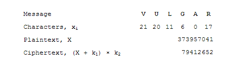
The first step involves parsing the message characters into numbers. For this step, A is labelled 0, B is 1, C is 2 … Y is 24, Z is 25 and space is 26.

Next, the characters are grouped into blocks of six characters. Each block of six characters will be converted into a number. The most straightforward method is to adopt a base-27 numbering system to represent the number where each character is a digit in the number. Expressed in base-10 (the same base that most humans use to interface with each other and with computers), the number is of the form
X = x₁ × 27⁵ + x₂ × 27⁴ + x₃ × 27³ + x₄ × 27² + x₅ × 27 + x₆
Where X is the plaintext and x_i is the i-th character in the block.

This X is part of the plaintext: the number which 6 characters of the message. The entire plaintext is made up of many different X’s to encode all the characters in the message.

To encrypt the plaintext X, some operation is performed on X to hide its original value:
C = (X + k₁) × k₂

k₁ and k₂ are predetermined constants. They are the cipher keys that are used to modify the plaintext. The result of the modification is the ciphertext, C.


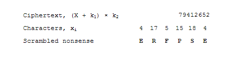
This ciphertext is then sent to the intended recipient. If anyone who intercepts the message attempts to convert the ciphertext into characters, they will be faced with a bunch of garbled characters.


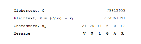
The intended recipient will have the correct cipher keys to unlock the message. To find the plaintext, the encryption operation is performed in reverse on the ciphertext:
X = (C / k₂) - k₁

To recover the x_i that would represent each character in the message, the recipient converts X to base 27 to recover the values x_i and therefore the message contents.

Option valuation- understanding how price volatility and duration to expiry affects the value of an option

This rather long article is laid out as follows:

Summary
Option fundamentals
Valuation approach
Relationship between profit from an option and the asset’s market price
The probable market price at exercise date of the option
How likely is it that I will profit from this option?
How much profit can I expect from this option?
Another example: on the money option
Volatility sensitivity of options
Valuing the option: a hand-waving approach

Summary:
The price volatility and duration affects options because of the asymmetrical way options payback the holder. High volatility implies a high likelihood for prices to move either up or down. If process move in one direction, the bond holder gains. If prices move in the opposite direction, the option holder does not suffer losses.
Thus, a larger price volatility and longer duration give will almost result in an increase in the value of the option.


Option fundamentals
Options are securities that grant the option holder the right to buy or sell an asset at a predetermined price some time in the future.

An example of an option to buy (a call option) would be an option to buy 100 barrels of crude oil for the price of US$ 7500 in December. The agreed upon price is called the strike price.
If in December, the market price for 100 barrels of crude oil increased to US$8000, the option holder will decide to exercise the option’s right to buy from the option writer at the cheaper price. Thus, the option holder’s profit is US$ 500.
However, if the price instead decreased to US$ 7000, the option holder will be better off buying in the market. So the option will not be exercised, and the option holder does not profit.

Therefore, the call option allows the holder to profit if the asset price increases, but does not result in losses if the asset price decreases. Of course, there is no free lunch; the option has to be purchased at a cost. We will discuss how the price volatility affects the cost of an option.


Valuation approach
The approach taken here is the estimate the expected return from the option position, then discount the value for risk.


Relationship between profit from an option and the asset’s market price

Returning to the above example, we can see that if the asset price is below the strike price, the call option holder does not suffer any losses. But if the asset price is above the strike price, the option holder can buy the asset at the strike price, and then sell the asset in the market at the market price, thus profiting from the difference between market and strike prices.

Figure 1 below shows the relationship between ending price and profit. Notice that if the ending market price is less than the strike price, there are no profit/losses. When ending market price is above the strike price, the profit is the difference between the strike price and the market price.


Figure 1


The probable market price at exercise date of the option

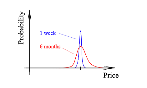
While we may be able to predict certain trends in the market, there will always remain a large element of uncertainty. Likewise, there is an uncertainty regarding the market price of the underlying asset at the expiry of the option. Two factors affect the uncertainty of market price at expiry date: duration to expiry, and volatility of the price.

If the option is to expire next week, and the market price today for 100 barrels of crude oil is US$ 7750, we would expect the price next week to be close to US$ 7750. The probability of a large change is small (but still present: a severe industrial accident in a major refinery could push prices up abruptly).

However, if the option is expiring in 6 months, there is more time for all sorts of market events to cause changes for the price of 100 barrels of oil to move away from the current price of US$ 7750.

In figure 2 below, we illustrate the probability of ending prices. As the graphs show, prices further in the future are more likely to move further from the current price.



Figure 2

The effect of price volatility is similar: assets which are more prone to fluctuation will have a more spread out probability density function than assets which have more stable prices.


How likely is it that I will profit from this option?

Earlier, we have shown that the profit from a call option position is asymmetrical: the holder profits if the asset price is above the strike price, but does not lose if the asset price is below the strike price.

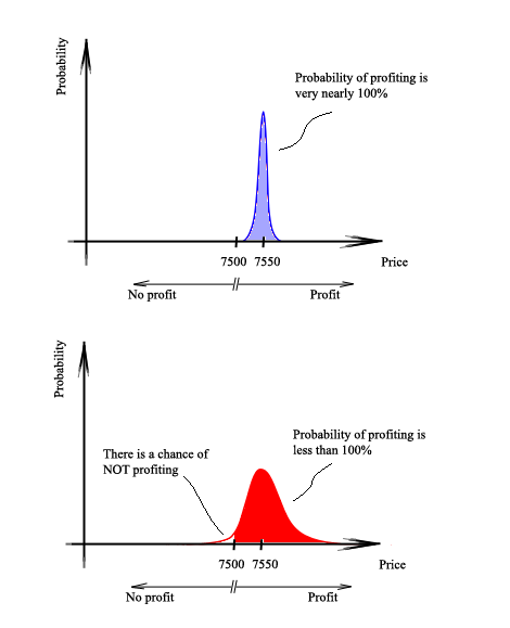
Let’s say the current asset price is 7750, and the strike price is set at 7500. We have two options, one that expires in one week, and one that expires in 6 months. If we were able to exercise NOW, we would definitely gain 250 in profits. But what about 1 week or 6 months later?

Figure 3 below shows that for the one-week option, we will almost certainly be in a profitable position. However, there is a chance of not being profitable if we take the 6-month option. This is because the longer duration increases the likelihood of the asset price moving below the strike price (however, we must not forget that the asset price can also move up higher).




Figure 3


Of course, this is not the end of our analysis. While we can now estimate the likelihood of making a profit, we still need to have a feel of how much we can expect to profit.


How much profit can I expect from this option?

If we are interested in estimating the expected profit from an option position, we need to find the total of the (probability of a particular asset price × the profit at that asset price) for all possible asset prices.

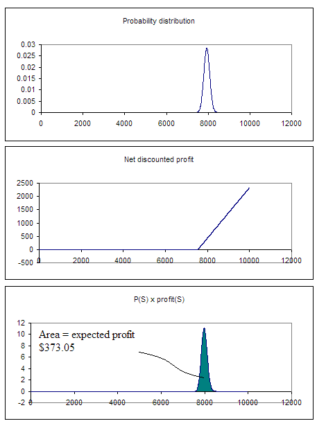
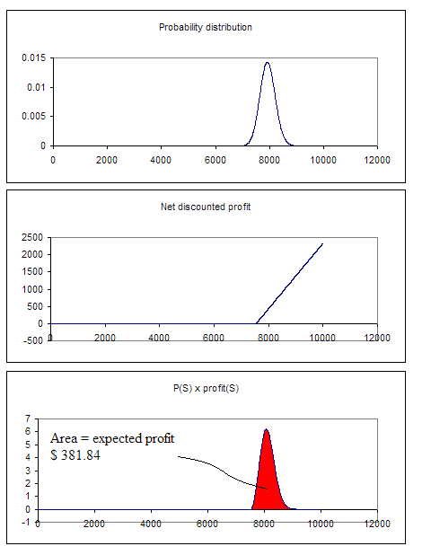
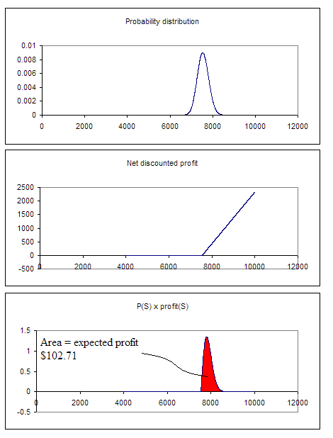
The expected profit from this position is the area below the (probability of a particular asset price × the profit at that asset price) curve. For the position of options expiring in 1 week and 6 months, the calculations are displayed graphically below (these calculations cannot be solved geometrically in a practical manner; a spreadsheet was required to calculate the probability density function, multiply the probability with the profit, and then calculated the area).



Figure 4


Figure 5

If we compare expected profit and likelihood of profit, we see that the 6 months position has a small likelihood of not profiting (as shown in figure 3) but greater expected profit. This is due to the fact that the 6 month option can earn large profits if the underlying price moves upwards significantly, but make no losses if the price goes below the strike price.


Another example: on the money option

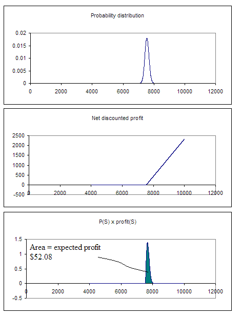
The sensitivity of an option’s value to price volatility and duration is particularly severe for an on the money option. This is an option which has a strike price equal to the current underlying price. We use the same examples as above, but this time the strike price is the same as the current price. If prices move up the slightest bit, the option holder will profit, but if prices move down the slightest bit, option holders will not lose money.



Figure 6



Figure 7


Volotility sensitivity of options

If we were to compare the sensitivity of options, we can see that an on the money option is very sensitive to a change in volatility (in the examples in figures 6 and 7, the expected profit jumps from 52.08 to 102.71, a 97% leap) while an in the money option is less sensitive (in the examples in figures 4 and 5, the expected profit jumps from 373.05 to 381.04, a mere 2% incement).

If an option was deeply out of the money (the strike price is well below the current underlying price), then we expect the option to expire without turning us any profit. Unless we have a massive increase in volatility, the value of this option will be very close to zero regardless of volatility.


Valuing the option
If the option holder is completely indifferent to risk, then the option holder will be willing to pay the expected value of the option in order to own the option.

However, this does not apply in the real world: buyers want to be reimbursed for risk. Thus, buyers will not be willing to pay the full expected value for an option with uncertain returns.

For options that are deeply in or out of the money, the option price will be very close to the expected profit. For in deeply in the money options, the expected profit is equal to the difference between the strike price and current market price (this is also equal to the area under the probability × profit curve). For deeply out of the money options, the expected profit is zero.

For options that have their probability functions straddling the strike price, the option price has to be adjusted for that fact that there could be decent profits or none at all. For volatile or long duration options (figure 7), we will expect the discount to be substantial; for less volatile and shorted duration options (figure 6), the discount will be less.

Deriving the present value of a fixed-payment annuity of finite life (not a perpetuity)

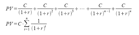
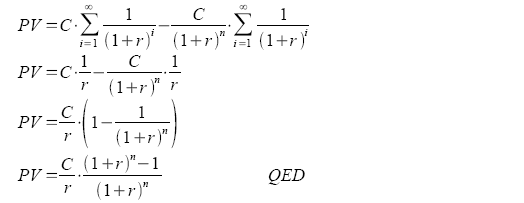
Many finance text books will provide the formula for the present value of such an annuity as the following:

Where C is the payment made every period, r is the discount rate to be applied, and n is the number of periods.

Unfortunately, elementary finance text books have a distasteful habit of presenting equations with no proof. The reader can either believe it, or sod it.

Here, we will derive the above equation.


The present value of an annuity is the sum of the discounted payments, as follows.

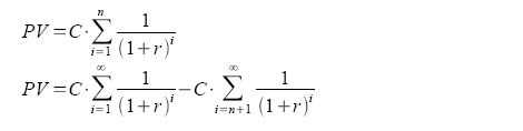
This sum can be expressed as the difference between two infinite sums (perpetuities) starting at different times:

Notice that the second perpetuity starts at n+1. We then modify the second perpetuity's notation so that the index starts from 1:

From studies of the present value of perpetuities, we know that the following is true:
*The derivation of this is attached as an appendix.

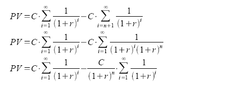
Substituting the above equation into our present value of an annuity:



Appendix – deriving the present value of a perpetuity

A perpetuity is an endless stream of fixed payments occurring at fixed intervals.

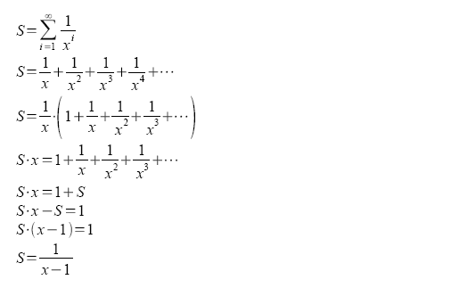
Its present value can be computed as follows:

The value of the infinite sum can be expressed as follows:
For simplicity, 1+r is replaced with x.

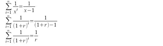
When we replace x back with 1+r, the equation becomes

Substituting our result into the present value of a perpetuity:

It seems that I have made a difference in the universe. While not a massive feat, it's definitely non-trivial.

The god-sister wrote:

As I plump myself into the back seat of my friend’s car on the way home from tuition and with my left cheek touching the cold surface of the car’s window, I thought about the boring-to-you-yet-interesting-to-me identity numbers. This was passed down to me by my great mathematics teacher who also happens to be my god brother, Tan Yee Wei (aka the Pink Man).

[Future reference for self when I get amnesia: Identity numbers are numbers that leave another number unchanged when an operation is applied. Yeah, I think that’s what he said. It seems so much less magical now that I’ve learnt in school. But a few years back when algebra was foreign to me, it was simply fascinating. He told me that the identity of addition (and subtraction) operations is 0 whereas the identity number for multiplication (or division) is 1. It’s simple really, if you add any number by 0, or subtract for that matter, you get the same number, thus 0 is the identity. And if you multiply or divide a number by 1, you’d also find yourself with the same number you started off with. Cool eh? Yes. I’m a dweeb. And come to think about it, I still find it quite fascinating. I mean, who would ever think about that sort of things?]

Well, that gave me a jump-start and got my mind churning. I realise that I have this hunger for knowledge. I love to inquire as I feast on information. As a matter of fact, I tend to be in favour of self-realizations. Likewise, I find myself always wanting to be the best that I can be.

Beauty in an ordered set plantation

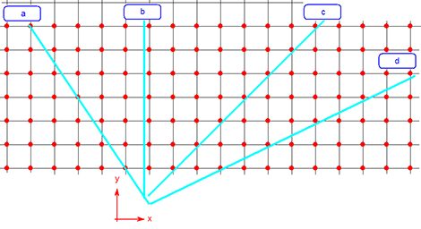
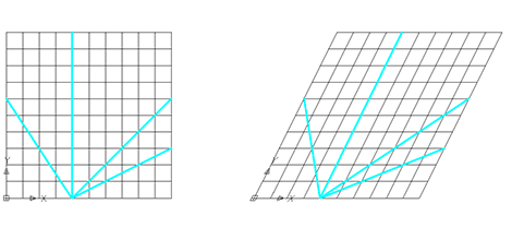
When driving along large, well ordered plantations, one often notices that the trees appear to line up in straight lines when one looks in different directions. The simplest example will be using a square grid as follows:


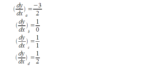
As the observer looks along the directions a, b, c, and d, he sees neat rows where tree trunks lined up. The directions a, b, c and d can start to make more sense when we express the gradient of the lines-of-sight:

We start with line d, for that is the simplest to explain:


This is derived by observing that y increases by one step when x increases by 2 steps. Similarly, the gradients for the other lines are:


The above shows that lines of sights with integer numerators and integer denominators will have ordered rows of trees. However, it should be noted that 2/2 is equal to 1/1, thus some integer-pairs need to be eliminated. This can be done by dividing both the numerator and denominator by all their common factors. In other words, the numerator and denominator is to be relatively-prime.

At this point, the argument is starting to look remarkably similar to the well known problem of “how many rational numbers are there?” The answer is infinity.

Thus, in an infinitely large plantation with trees of infinitesimally narrow trunks (this is a necessary condition to prevent other trees' trunks from blocking the line of sight), there are infinitely many lines of sights that result in orderly lines. Of course, it is naturally assumed that in this odd plantation, the spacing and arrangement of trees are perfectly regular.

The strength of the visible trend line of lined-up trees depends on how far one needs to move along the line of sight before another tree is sighted. In other words, the visibility of the trend line is dependent on the linear density of the trees along the line of sight.

The packing density can be inferred by the numerator and denominator of the gradient (when already expessed as relatively-prime numbers). The separation distance of trees along the line of sight is simply the hypotenuses of the triangle consisting of the perpendicular sides of lengths [numerator] and [denominator]. The separation distance is thus:



Thus, for a line of sight to be a very obvious one, both x and y must be small to result in more trees occurring along the line of sight. This is consistent with general observations in the field that the line of trees along the line of sight b is more obvious than the line along c, which is more obvious than along d, which is more obvious than along a.



This approach to analysis can apply to non-orthogonal layouts as well. For example, if the grid was deformed as follows, the analysis above still applies.


However, inference of the strength of the trend line requires explicit coordinate manipulation to determine the exact inter-tree spacing (the equation of s=sqrt (x^2 + y^2) does not apply for non-orthogonal x and y).


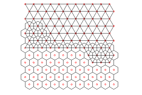
If the plantation was arrayed in a hexagonal/triangular layout (which allows the greatest packing density of trees), the above analysis can still be used. (note: in this arrangement, trees can be the vertices of the triangles, of the the centres of hexagons. This is illustrated below)


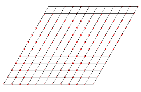
The hexagonal/triangular layout can be recast as a deformed square (properly called a parallelogram), as shown below:

What is the matrix?

The god-sister was having conceptual trouble with matrices. We can’t blame her; the mathematics text books we use do not justify the importance of matrices.

Today, I received a simple message from her:
PS. I get matrices. Thanks!

Perhaps it would be useful to make the material publicly available.


***

The following shows one aspect of how matrices are damn useful.
It might appear magical, that the two solution methods below manage to produce the same result. It is not magic.

Matrices were designed by humans. They were designed to have certain properties (the main one being: for multiplications, sum the products of row and column elements).
Matrices and matrix manipulation rules were designed so that they would be useful. If a matrix operation was defined with some stupid rule (like when you multiply two matrices, you multiply each number with the other number, and then add the number of days in your menstrual cycle) then matrices will be of no mathematical use.



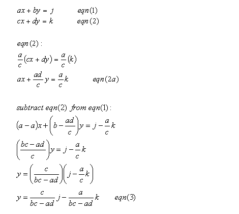
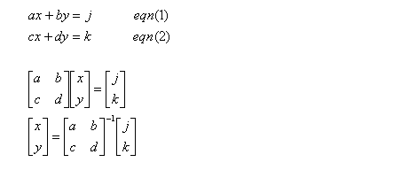
Lets have two equations:
The coefficients a, b, c and d are known. The constants j and k are also known. We want to find the values of x and y that would satisfy these equations.

A typical way to solve this is as follows:
Multiply equation (2) with a suitable number so that the coefficient for x is the same as in equation (1).
Then subtract equation (2) from (1). From this step, we will be able to solve for y. With y known, we then put y into one of the equations to find x.

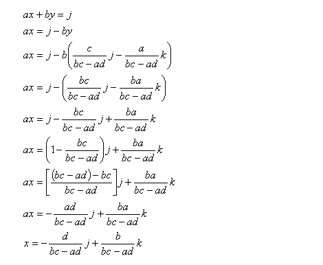
Sticking to the symbols (so we can have a general solution that would work with any a, b, c, d, j and k):



Now, in equation (1), y is now expressed as known numbers. Therefore, y is now solved. We now replace y into equation (1):


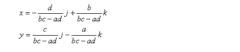
Because we are long winded, we will repeat our results:


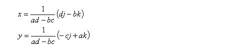
We will also rearrange the results for future convenience:



If we were to solve this pair of equations using a matrix, the procedure applies:

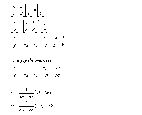
To inverse a 2-by-2 matrix:
Therefore:


The results match the result we obtained from the above equation manipulation. And it’s much faster, no?

Variance and covariance of a weighted portfolio

You should not be reading this post; shoo, get a life.


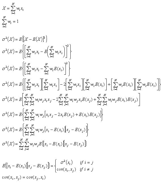
Was fiddling with some equations on my flight from Shanghai and Tianjin, and the following came about. The stuff I found in the text was unsatisfactorily complicated and not generalised enough.



I think the most conceptually challenging part of the preceding definition of variance lies in the sudden appearance of the index j (this appears on line 5). A brief illustration follows, showing how the additional index is summoned:

Deriving the first partial derivatives of the Black-Scholes call price equation

Material presented here will be used to discuss hedging strategies to simultaneously hedge an options portfolio against various exposures.

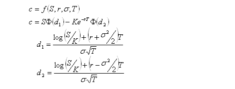
The call option price:


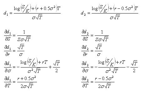
The partial derivatives of d1 and d2:


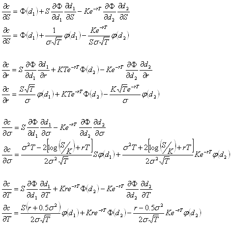
Partial differentiating c with respect to each variable:


And we're done for today. Easy, no?

Hedging strategies: a mathematical treatment of delta, delta-gamma, and third-order hedging

Some knowledge of options and delta hedging is required. This post is intended to demonstrate various concepts that will be used in a future post. All price-derivatives of the value of a call option have been derived previously here.


The objective of hedging is to maintain the value of a portfolio in an uncertain market. In hedging against changes in asset prices, a portfolio consisting of options and underlying asset is arranged so that if the value of the asset decreases, the value of the options will increase. The result is a portfolio value that will change by a small amount if the underlying asset price changed.

In today’s analysis, portfolios are created consisting of:
-long positions in the underlying asset, and
-short positions in call options.


The change in value of a portfolio due to a change in the asset price can be expressed as follows:



This equation has infinitely many terms, but an approximation can be made by retaining only as many terms as desired. Because the objective of hedging is to maintain the portfolio value constant regardless of any change in S, the following condition needs to be satisfied for all values of i:



In delta hedging, only the first term is retained for accuracy to the first-order:



In delta-gamma hedging, the first two terms are retained for second-order accuracy:



For third-order accuracy,



A portfolio consisting of long positions in the underlying asset and short positions in call options would have the following value:

where w corresponds to the quantity of each asset type in the portfolio.



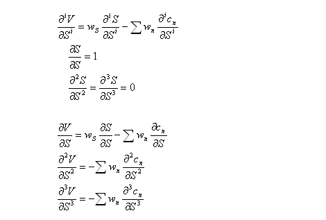
Similarly, the first, second and third derivatives of portfolio value with respect to asset price are:



Delta hedging
For delta hedging, only one kind of call option is required to hedge the portfolio. The value of the portfolio is to be V, and the weighted sum of first derivatives is to be zero:



Thus, the number of stocks and options to be purchased is the solution to the following matrix equation:



Delta-gamma hedging
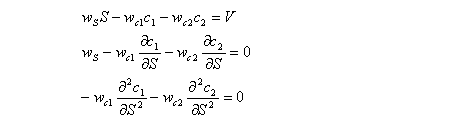
For delta-gamma hedging, two kinds of call option are required to hedge the portfolio. The value of the portfolio is to be V, and the weighted sums of first and second derivatives are to be zero:



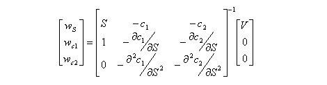
Thus, the number of stocks and options to be purchased is the solution to the following matrix equation:



Third-order hedging
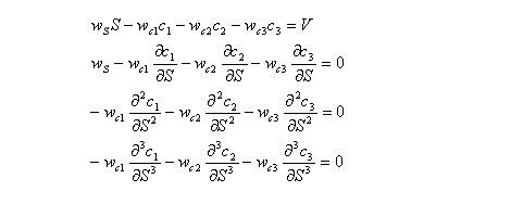
For hedging to the third order, three kinds of call option are required to hedge the portfolio. The value of the portfolio is to be V, and the weighted sums of first, second and third derivatives are to be zero:



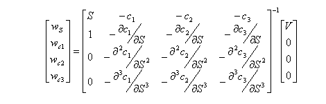
Thus, the number of stocks and options to be purchased is the solution to the following matrix equation: