Finally putting things into practice

I have been unable to access any blogspot sites since Friday, a remarkable coincidence with my little outburst against the local government regime. Perhaps they are related?

Anywhere else and I’d have said bullshit, but this country has proven itself at being able to throw up unpleasant surprise after unpleasant surprise after unpleasant surprise.


***

In the intervening time, I have FINALLY taken the time to actually start some financial planning. Like what the texts books have been telling me since… June 2007.

1. Identify financial needs and goals
2. Allocate assets

In line with item 1, I did a budget forecast of my next big thrust into fatherhood dictatorship, and the initial results were not encouraging. 10,000 AUD just to secure a miserable seat in the Outer Party’s Supervisory Committee is just… depressing.

How the fish do these crooks finance themselves into the Inner Party Censorship Board and Economic Planning Council? Ok fine, stupid question: they are crooks.


The asset allocation bit was a bit trickier. Having made earlier contributions to various mutual funds, I had to break down each fund into its constituent asset types to find my total exposure to each asset type. Then compare the existing allocation to the target allocation etc etc.


Ok I’ll not bore you with the number-crunching and data manipulation game.

Doom and gloom: my first economic downturn1

For the past two working weeks, I had been in Shenzhen² for some work-related affairs, returning to Shanghai for the weekends and Mondays. Both the workplace and accommodation had no internet access, thus cutting me off from the universe at large.

While at Shenzhen, I witnessed a company in the midst of downsizing. It was unpleasant yet morbidly fascinating, like how motor accident would draw curious onlookers.

The company retrenched approximately 2/3 of its staff and moved out of its rented office to operate from a flat. With the severe downsizing of staff, much of the company’s assets became redundant, including the company car, several computers, a handful of air conditioners and furniture.

Departing staff made cash offers for these items, knowing full well the management will not have the time or connections to sell them. Eventually they were sold at prices well below the items’ book values, with computers being sold for a meagre 500 RMB apiece and the split unit air conditioners, 300 RMB.

One of the more street smart employees told the general manager that his friends wanted to buy the computers too – obviously he was aware that of the arbitrage opportunity at hand. The general manager was quick enough to say the original price of 500 was for the staff member; other buyers would have to pay the ‘full price’ of 800. This was still agreeable to the arbitrageur, and he went away with 4 workstations and the company car for an undisclosed sum.

On the last 2, 3 working days for the retrenched staff, the motivation for (pretending to) work had clearly evaporated. They grouped together chit-chatting, watching videos, reading comics and surfing the net.

Even with the substantially reduced rental and salary costs, all is not rosy. The company is already committed to investments that require further capital before turning a profit, yet the company is barely making it for the month’s salary and retrenchment remuneration³.


----

1. I was too young in 1987 and 1998 to notice with much clarity
2. location name changed
3. Chinese labour law requires that employers pay retrenched employees one month’s pay for each full year employed.

Option valuation- understanding how price volatility and duration to expiry affects the value of an option

This rather long article is laid out as follows:

Summary
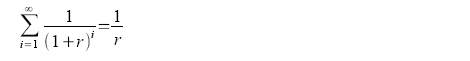
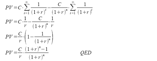
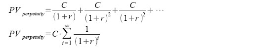
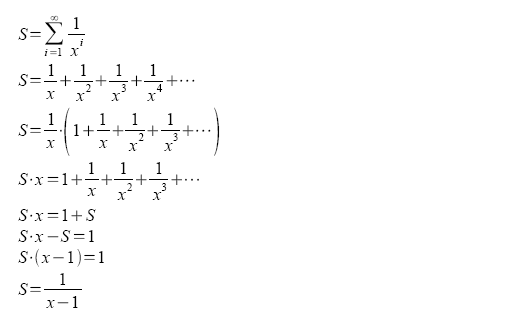
Option fundamentals
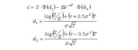
Valuation approach
Relationship between profit from an option and the asset’s market price
The probable market price at exercise date of the option
How likely is it that I will profit from this option?
How much profit can I expect from this option?
Another example: on the money option
Volatility sensitivity of options
Valuing the option: a hand-waving approach

Summary:
The price volatility and duration affects options because of the asymmetrical way options payback the holder. High volatility implies a high likelihood for prices to move either up or down. If process move in one direction, the bond holder gains. If prices move in the opposite direction, the option holder does not suffer losses.
Thus, a larger price volatility and longer duration give will almost result in an increase in the value of the option.


Option fundamentals
Options are securities that grant the option holder the right to buy or sell an asset at a predetermined price some time in the future.

An example of an option to buy (a call option) would be an option to buy 100 barrels of crude oil for the price of US$ 7500 in December. The agreed upon price is called the strike price.
If in December, the market price for 100 barrels of crude oil increased to US$8000, the option holder will decide to exercise the option’s right to buy from the option writer at the cheaper price. Thus, the option holder’s profit is US$ 500.
However, if the price instead decreased to US$ 7000, the option holder will be better off buying in the market. So the option will not be exercised, and the option holder does not profit.

Therefore, the call option allows the holder to profit if the asset price increases, but does not result in losses if the asset price decreases. Of course, there is no free lunch; the option has to be purchased at a cost. We will discuss how the price volatility affects the cost of an option.


Valuation approach
The approach taken here is the estimate the expected return from the option position, then discount the value for risk.


Relationship between profit from an option and the asset’s market price

Returning to the above example, we can see that if the asset price is below the strike price, the call option holder does not suffer any losses. But if the asset price is above the strike price, the option holder can buy the asset at the strike price, and then sell the asset in the market at the market price, thus profiting from the difference between market and strike prices.

Figure 1 below shows the relationship between ending price and profit. Notice that if the ending market price is less than the strike price, there are no profit/losses. When ending market price is above the strike price, the profit is the difference between the strike price and the market price.


Figure 1


The probable market price at exercise date of the option

While we may be able to predict certain trends in the market, there will always remain a large element of uncertainty. Likewise, there is an uncertainty regarding the market price of the underlying asset at the expiry of the option. Two factors affect the uncertainty of market price at expiry date: duration to expiry, and volatility of the price.

If the option is to expire next week, and the market price today for 100 barrels of crude oil is US$ 7750, we would expect the price next week to be close to US$ 7750. The probability of a large change is small (but still present: a severe industrial accident in a major refinery could push prices up abruptly).

However, if the option is expiring in 6 months, there is more time for all sorts of market events to cause changes for the price of 100 barrels of oil to move away from the current price of US$ 7750.

In figure 2 below, we illustrate the probability of ending prices. As the graphs show, prices further in the future are more likely to move further from the current price.



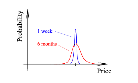
Figure 2

The effect of price volatility is similar: assets which are more prone to fluctuation will have a more spread out probability density function than assets which have more stable prices.


How likely is it that I will profit from this option?

Earlier, we have shown that the profit from a call option position is asymmetrical: the holder profits if the asset price is above the strike price, but does not lose if the asset price is below the strike price.

Let’s say the current asset price is 7750, and the strike price is set at 7500. We have two options, one that expires in one week, and one that expires in 6 months. If we were able to exercise NOW, we would definitely gain 250 in profits. But what about 1 week or 6 months later?

Figure 3 below shows that for the one-week option, we will almost certainly be in a profitable position. However, there is a chance of not being profitable if we take the 6-month option. This is because the longer duration increases the likelihood of the asset price moving below the strike price (however, we must not forget that the asset price can also move up higher).




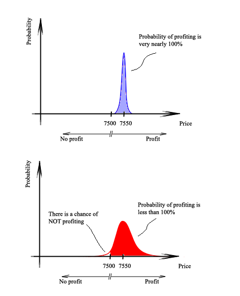
Figure 3


Of course, this is not the end of our analysis. While we can now estimate the likelihood of making a profit, we still need to have a feel of how much we can expect to profit.


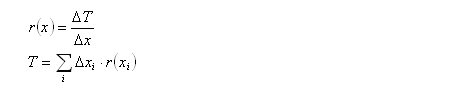
How much profit can I expect from this option?

If we are interested in estimating the expected profit from an option position, we need to find the total of the (probability of a particular asset price × the profit at that asset price) for all possible asset prices.

The expected profit from this position is the area below the (probability of a particular asset price × the profit at that asset price) curve. For the position of options expiring in 1 week and 6 months, the calculations are displayed graphically below (these calculations cannot be solved geometrically in a practical manner; a spreadsheet was required to calculate the probability density function, multiply the probability with the profit, and then calculated the area).



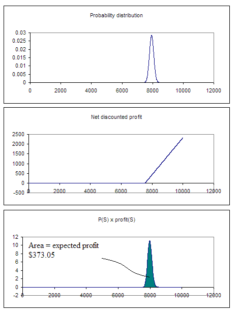
Figure 4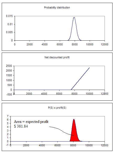


Figure 5

If we compare expected profit and likelihood of profit, we see that the 6 months position has a small likelihood of not profiting (as shown in figure 3) but greater expected profit. This is due to the fact that the 6 month option can earn large profits if the underlying price moves upwards significantly, but make no losses if the price goes below the strike price.


Another example: on the money option

The sensitivity of an option’s value to price volatility and duration is particularly severe for an on the money option. This is an option which has a strike price equal to the current underlying price. We use the same examples as above, but this time the strike price is the same as the current price. If prices move up the slightest bit, the option holder will profit, but if prices move down the slightest bit, option holders will not lose money.



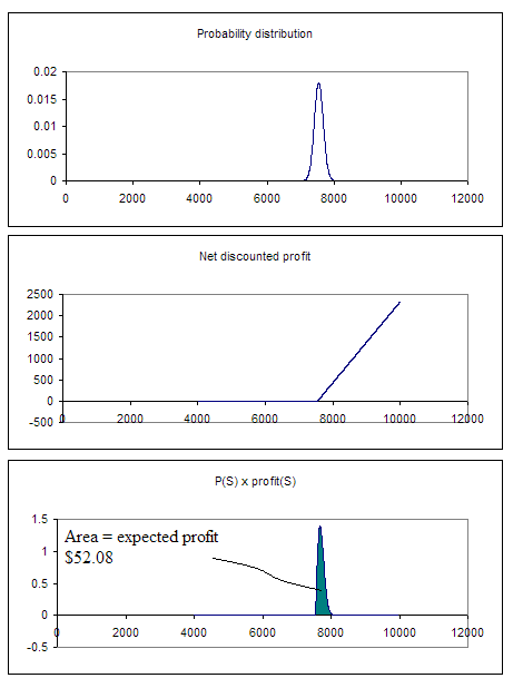
Figure 6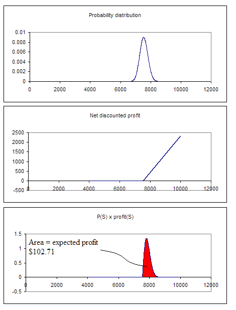



Figure 7


Volotility sensitivity of options

If we were to compare the sensitivity of options, we can see that an on the money option is very sensitive to a change in volatility (in the examples in figures 6 and 7, the expected profit jumps from 52.08 to 102.71, a 97% leap) while an in the money option is less sensitive (in the examples in figures 4 and 5, the expected profit jumps from 373.05 to 381.04, a mere 2% incement).

If an option was deeply out of the money (the strike price is well below the current underlying price), then we expect the option to expire without turning us any profit. Unless we have a massive increase in volatility, the value of this option will be very close to zero regardless of volatility.


Valuing the option
If the option holder is completely indifferent to risk, then the option holder will be willing to pay the expected value of the option in order to own the option.

However, this does not apply in the real world: buyers want to be reimbursed for risk. Thus, buyers will not be willing to pay the full expected value for an option with uncertain returns.

For options that are deeply in or out of the money, the option price will be very close to the expected profit. For in deeply in the money options, the expected profit is equal to the difference between the strike price and current market price (this is also equal to the area under the probability × profit curve). For deeply out of the money options, the expected profit is zero.

For options that have their probability functions straddling the strike price, the option price has to be adjusted for that fact that there could be decent profits or none at all. For volatile or long duration options (figure 7), we will expect the discount to be substantial; for less volatile and shorted duration options (figure 6), the discount will be less.

Deriving the present value of a fixed-payment annuity of finite life (not a perpetuity)

Many finance text books will provide the formula for the present value of such an annuity as the following:

Where C is the payment made every period, r is the discount rate to be applied, and n is the number of periods.

Unfortunately, elementary finance text books have a distasteful habit of presenting equations with no proof. The reader can either believe it, or sod it.

Here, we will derive the above equation.


The present value of an annuity is the sum of the discounted payments, as follows.

This sum can be expressed as the difference between two infinite sums (perpetuities) starting at different times:

Notice that the second perpetuity starts at n+1. We then modify the second perpetuity's notation so that the index starts from 1:

From studies of the present value of perpetuities, we know that the following is true:
*The derivation of this is attached as an appendix.

Substituting the above equation into our present value of an annuity:



Appendix – deriving the present value of a perpetuity

A perpetuity is an endless stream of fixed payments occurring at fixed intervals.

Its present value can be computed as follows:

The value of the infinite sum can be expressed as follows:
For simplicity, 1+r is replaced with x.

When we replace x back with 1+r, the equation becomes

Substituting our result into the present value of a perpetuity:

Marginal production and average production

Note: This post is here because my girlfriend refuses to be impressed by my prowess in calculus.


In economics, the study of costs as a function of production quantity (or vice-versa) is one of the key considerations.

In many cases, it is desirable to know the production quantity that would give the greatest profit margin- this is the condition that gives the highest ratio of production to cost.

The marginal output curve is also of interest, because it will describes the effect of investing additional resources into the venture. Given that we are currently using so much resources to produce so much output, what additional benefit do we get from additional resources spent?

When the marginal output curves and average product (ratio of production to cost) curves are plotted on the same axes, the intersection of these two curves occur at the maximum ratio of production to cost.

This little observation (presented as a statement, without neither explanation or evidence) had disturbed me when I studied macroeconomics in 2002, and also disturbed me when I studied economics yesterday. When I wheeled out the unrivalled fire-power of calculus, all doubts crumbled.

Let x be the resources invested in the venture, and f(x) be the production output resulting from an investment of x.

The marginal production M(x) can be expressed as the first derivative of f(x) with respect to x, the average productions A(x) is the total production over the total cost.



When the average production is maximum, the gradient of A is zero. Therefore, the first derivative of A is equal to zero at the maximum average production.



QED.

Variance and covariance of a weighted portfolio

You should not be reading this post; shoo, get a life.


Was fiddling with some equations on my flight from Shanghai and Tianjin, and the following came about. The stuff I found in the text was unsatisfactorily complicated and not generalised enough.



I think the most conceptually challenging part of the preceding definition of variance lies in the sudden appearance of the index j (this appears on line 5). A brief illustration follows, showing how the additional index is summoned:

An introduction to income tax for the mathematically-inclined (calculus is required)

In almost all countries, the payable income tax depends on the individual’s taxable income earned in the financial year.

Generally, the tax rates are quoted as marginal rates for different income brackets. The Hong Kong marginal tax rates for different income levels is shown below:

The first $30,000 will be taxed at 2%
The 30,001st to 60,000th dollar will be taxed at 8%
The 60,001st to 90,000th dollar will be taxed at 14%
Subsequent income above $90,000 will be taxed at 20%

In this analysis of income tax, the concept of marginal tax is of great importance. At a marginal tax rate of 5%, each additional dollar earned will result in an additional 5 cents of tax.

We will now use the following notation: x is the income earned, and T is the total tax payable, and r is the marginal tax rate.

From the preceding statement, it is shown that the additional tax payable, ΔT, is a multiple of the tax rate, r, and the additional income, Δx:



As the above manipulation shows, the marginal tax rate is the rate of change of total payable tax with respect to income.

As the example of Hong Kong’s marginal rates, income is taxed at different rates. The first few thousand will generally be taxed at a very low marginal rate, and the subsequent thousands taxed at a higher marginal rates. To find the total tax payable (as any income earner would like to know), one procedure is to use the Riemann integral:



Essentially, what this shows is that each dollar earned will be taxed at the marginal tax rate that applies for that dollar. The total tax payable is the sum of all products of individual dollars and respective marginal tax rates.






A comparison between the above charts will verify that T(x) is the definite integral of r(x) with limits 0 and x. The slope of T(x) changes when r(x) changes, which is not surprising given that a greater marginal rate implies a faster increase in the total taxes.

As the marginal tax rate is always non-negative (many countries have a zero-tax bracket for the first thousands earned), the total tax payable increases monotonically with income. That is to say, and increase in income will NEVER cause a decrease in payable tax.

Because the tax payable is an integral of a continuously defined function, the tax payable is a continuous function. While the rate of increase of the payable tax might change due to a change in the marginal tax rate, the tax payable will never take a discontinuous jump. Thus in systems using the marginal tax rate system, there is no dramatic taxation advantage in earning a few dollars more/less to try to squeeze into a different tax bracket.


End note

In the system of taxes, money is can only exist in discrete quantities. Certain taxation systems will require income to be rounded to the closest dollar, others will accept the income quoted in dollars and cents. Regardless, there exists a smallest unit in which money can be counted, be it dollar or cent.

Thus, the use of discrete calculus would be proper instead of real (continuous) calculus as done above.

The differential equation r(x) = dT/dx will no longer apply, and the following will take its place:



where Δx is the discrete currency unit.

Nick Leeson and Jérôme Kerviel- a very brief comparison of billion-Euro rogue traders

The latest scandal to hit the financial news is a case of fraud at the French bank Société Générale involving sums of up to 4.9 billion Euros. The protagonist in the middle of this storm is Jérôme Kerviel, an equities derivatives trader.

This case immediately brings to mind the famed Nick Leeson, whose unauthorised speculative trades resulted in losses of 827 million Pounds and the collapse of Barings Bank in 1995.

So how does Kerviel compare against Leeson? The most straight-forward approach would be to compare the present value of the magnitude of their losses.

Leeson managed to lose 827m GBP 13 years ago. Arbitrarily assuming the average interest rate between 2005 and now to be 4% p.a., the present value of that sum is actually a staggering 1.4 billion Pounds.

827m * e^(0.04*13) = 1391m GBP

Kerviel, on the other hand, has managed to evaporate 4.9 billion Euros. However, there are reports suggesting Kerviel lost 1.5 billion; the other 3.4 billion Euros was the bank’s own (un)doing.

A rival investment banking executive said Mr Kerviel did not lose €4.9bn by trading futures on European share indices, as Soc.Gen. claims, but only €1.5bn – the deficit his trading had accumulated by the time he was caught.

"The board of SocGen lost the other €3.4bn," said the rival banker. But the bank defended its actions, saying it could not risk keeping the positions open.

source

Now, how does Kerviel’s 1.5 billion Euros compare to Leeson’s present value of 1.4 billion Pounds?

Using today’s exchange rate of 0.74 Pounds to the Euro, Kerviel’s losses of 1.5 billion Euros is equivalent to 1.11 billion Pounds. Given the very rough estimation methods in this assessment, this figure of 1.11 billion Pounds is not remarkably different to what Leeson managed (1.4 billion Pounds).


***

Like the title already says, "very brief." Visit the Financial Times for a more details.

Deriving the first partial derivatives of the Black-Scholes call price equation

Material presented here will be used to discuss hedging strategies to simultaneously hedge an options portfolio against various exposures.

The call option price:


The partial derivatives of d1 and d2:


Partial differentiating c with respect to each variable:


And we're done for today. Easy, no?

Hedging strategies: a mathematical treatment of delta, delta-gamma, and third-order hedging

Some knowledge of options and delta hedging is required. This post is intended to demonstrate various concepts that will be used in a future post. All price-derivatives of the value of a call option have been derived previously here.


The objective of hedging is to maintain the value of a portfolio in an uncertain market. In hedging against changes in asset prices, a portfolio consisting of options and underlying asset is arranged so that if the value of the asset decreases, the value of the options will increase. The result is a portfolio value that will change by a small amount if the underlying asset price changed.

In today’s analysis, portfolios are created consisting of:
-long positions in the underlying asset, and
-short positions in call options.


The change in value of a portfolio due to a change in the asset price can be expressed as follows:



This equation has infinitely many terms, but an approximation can be made by retaining only as many terms as desired. Because the objective of hedging is to maintain the portfolio value constant regardless of any change in S, the following condition needs to be satisfied for all values of i:



In delta hedging, only the first term is retained for accuracy to the first-order:



In delta-gamma hedging, the first two terms are retained for second-order accuracy:



For third-order accuracy,



A portfolio consisting of long positions in the underlying asset and short positions in call options would have the following value:

where w corresponds to the quantity of each asset type in the portfolio.



Similarly, the first, second and third derivatives of portfolio value with respect to asset price are:



Delta hedging
For delta hedging, only one kind of call option is required to hedge the portfolio. The value of the portfolio is to be V, and the weighted sum of first derivatives is to be zero:



Thus, the number of stocks and options to be purchased is the solution to the following matrix equation:



Delta-gamma hedging
For delta-gamma hedging, two kinds of call option are required to hedge the portfolio. The value of the portfolio is to be V, and the weighted sums of first and second derivatives are to be zero:



Thus, the number of stocks and options to be purchased is the solution to the following matrix equation:



Third-order hedging
For hedging to the third order, three kinds of call option are required to hedge the portfolio. The value of the portfolio is to be V, and the weighted sums of first, second and third derivatives are to be zero:



Thus, the number of stocks and options to be purchased is the solution to the following matrix equation:

Deriving the exact equations for Delta, Gamma and the unnamed third price-derivative of a call option

An underlying knowledge of options is assumed. This post is intended to demonstrate various parameters that will be used in a future post.

Using the Black-Scholes model for options pricing, a call option price is:

Where Φ(x) is the cumulative probability function of a standardised normal variable.


Using partial derivatives, the rate of change of c with respect to S will be derived. This rate of change is commonly labelled Δ, Delta.



The normalised probability function and cumulative probability function are related in the following manner:



Substituting this into the partial derivative of c, the following results:



Further manipulation of the above equation can yield the second derivative of c with respect to S, commonly labelled Gamma or Γ.



The standardised normal probability distribution function and its derivative are of the following form:



Substituting the derivative of the normal probability distribution function into the second derivative of c with respect to S,

Click here to see skipped steps in this derivation


The third derivative of C with respect to S is not given a Greek symbol. Using the above result,

Click here to see skipped steps in this derivation


In summary,