Hydrodynamics for noobs

Seeing that my work load is particularly low today, I’ll attempt to clarify some fundamental concepts regarding the flow of water¹ through pipes and fittings.

A very fundamental notion to understand in hydraulics is the relationship between flow speed and pressure. A partially blocked pipe will be used to illustrate this relationship.



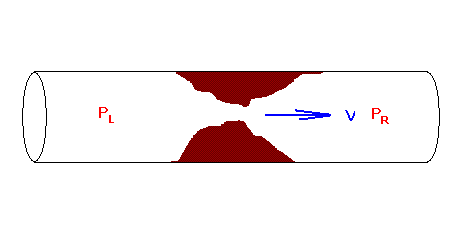
In this example, the pressure on the left, P_L, is greater than the pressure on the right, P_R. This pressure difference will accelerate water through the blockage, from left to right. As the speed of water flow increases, friction also increases. This friction force is proportional to the square of velocity: doubling the velocity results in four times the friction; tripling the velocity results in nine times the friction.
The flow of water will continue to increase until such a flow speed where the pressure difference, P_L - P_R is balanced by the friction of water rushing through the narrow blockage.

Instead of expressing the friction/ flow resistance as a friction force, it is commonly expressed as a pressure difference between the upstream and downstream areas, as a function of flow speed.

ΔP = kV²

This approach to expressing flow resistance is very convenient for practical problems. For example, one may wish to pump a certain volume of water through a valve into a water tank. If the desired flow speed V is known, and the valve’s value of k is known, the pressure difference between the valve’s front and back can be determined. Knowing the pressure inside the water tank, the pressure before the valve needs to be greater than the tank’s pressure by ΔP. This approach also can be used if there are several valves: the pressure difference across the valves can be added together to find out the total pressure loss that occurs when water flows through the system.


What happens when you open a valve in a water tap?

For simplicity, we will assume the water source for a tap is at a constant pressure, and the tap opens out to atmospheric pressure. This is quite a reasonable assumption, especially if the tap is connected directly to a water tank with very minimal lengths of piping.

As is the case for water taps, opening the valve allows water to flow out of the tap. Water flows from the high pressure side through the valve and out to the low pressure side. The flow speed is limited by the tap’s flow resistance k.

As shown above, the flow speed and pressure difference is related by ΔP = kV². Given that the pressure difference does not change, the only way to regulate the quantity of water coming out of the tap is by changing k. This happens when the valve is opened or closed. When the valve is closed, k increases (completely closed, the value of k is infinity- there is zero flow even when pressure difference is a finite quantity). When the valve is opened, k decreases.

Notes:
1. or any other viscous and incompressible fluid

Fun with the MoTeC data interpreter

What I did for Valentine’s Day:
Played GTR 2 for a few hours.

GTR 2 is a fearsomely realistic racing simulator based on the 2003 and 2004 FIA GT Championship series. While there are a huge number of bells and whistles, one of the most fascinating features of the game is the ability to save the car data into a MoTeC log file.

This is the same file format that a MoTeC data logger on an actual race car will produce: a time history of individual wheel speeds, suspension positions, suspension speeds, engine revs, throttle position, brake pedal pressure, steering angle, longitudinal acceleration, lateral acceleration, individual tyre temperatures at the inside, centre and outside areas…

And with the MoTeC data interpreter program, magic is possible.


***

The user can perform various mathematical operations on any combination the generous set of data logged by the MoTeC data logger.

For example, the instantaneous radius of curvature of the vehicle’s path can be calculated by rearranging the following equation:
a = v²/r
r = v²/a

Both the vehicle speed and lateral acceleration are measured, and so the radius can be determined.

Even more interesting, a general relationship between the vehicle’s speed and aerodynamic downforce can be observed after the data is suitably processed.

The principle objective of demanding greater aerodynamic downforce in a racing car is to allow greater acceleration (both in the longitudinal and lateral directions). Consequently, greater downforce will allow the vehicle to have higher accelerate.

From the logged longitudinal and lateral accelerations, the acceleration magnitude of the vehicle can be determined:
|a| = sqrt( a_long² + a_lat²)

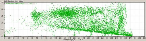
When |a| is plotted against vehicle velocity, the following scatter plot appears:



Click here for large size image

x axis: vehicle speed, v (km/h)
y axis: acceleration magnitude, |a| (g)
This plot consists of data recorded over a distance of 6 laps, equivalent to a duration of 13 minutes. Data was recorded at 10 Hz, producing 8130 data points.

Two general trends are visible:
the lower trend, consisting of a straight line that indicates a decreasing acceleration at higher speeds
the upper trend, indicating the maximum achievable acceleration increases when vehicle speed increases

The lower trend line corresponds to data recorded when the vehicle is accelerating on straight sections of the track. Given that the power output of the engine is maintained near the peak output (by adjusting the gearbox ratios to suit the track), the straight line is consistent with the fact that an object accelerated with a constant power will accelerate slower when the object is moving at a faster speed.

The upper trend is not as clear, but is nonetheless visible as an upward sloping trend.
At 60 km/h, |a| is approximately 1.75 g.
At 100 km/h, |a| is approximately 1.85 g.
At 160 km/h, |a| is approximately 2.10 g.
At 260 km/h, |a| is approximately 2.25 g.

Several data samples plot outside the upper trend because dips and bumps in the track will result in a different normal force acting on the wheels, thus allowing momentary increases and decreases in absolute acceleration.

A small cluster of data at 250 km/h show substantial deviation from the upper limit of acceleration. This, too, is caused by changes in track elevation where the main straight slopes upwards.


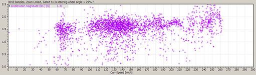
A similar plot can be produced showing lateral component of acceleration instead of total acceleration. In this case, |a_lat| was plotted against vehicle speed.

To prevent the chart from being cluttered with data not related to lateral acceleration (on straights, the lateral component of acceleration is close to zero), the plot was gated by plotting only data points that meet certain criteria.

Here, a new expression was defined, where
Steering = if (steering wheel angle > 25%) 1; else 0;

This expression will take the value 1 if there is substantial steering input, and 0 otherwise.

The criteria for gating the data is then set such that only data points with steering = 1 will be plotted, resulting in the scatter plot below:



Click here for large size image

x axis: vehicle speed, v (km/h)
y axis: lateral acceleration magnitude, |a_lat| (g)
This plot consists of data recorded over a distance of 6 laps, equivalent to a duration of 13 minutes. Data was recorded at 10 Hz, producing 8130 data points. Of these, 3042 data points satisfied the gating criteria and were plotted.

The |a_lat| plot resembles the |a| plot, except for the absence of the lower trend line. This is expected, because the lower trend line is associated with longitudinal acceleration driven by the vehicle’s engine.

A trend line indicating the upper bound of acceleration magnitude was constructed by approximation, and the following correlation appears:
|a|_max = 0.0017 V + 1.56,
The units for |a|_max and V are g and km/h respectively.


With the correlation between maximum |a| and vehicle speed approximated, a new variable called theoretical max acceleration was defined
theoretical max acceleration = 0.0017 vehicle speed + 1.56
This variable indicates the maximum acceleration that the vehicle tyres can provide.

When the instantaneous values of the theoretical max acceleration is compared against the actual accelerations, it can show areas where the driver can improve his/her lap time. For example, it can reveal that the driver can apply the brakes slightly later and harder on entry into a particular corner, thus shaving several milliseconds from the lap time; or that the vehicle can move slightly faster at a particular curve without exceeding the traction limits of the tyres.

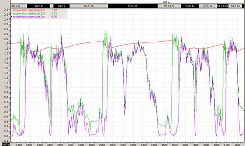
In the following graph, theoretical max acceleration is plotted together with actual |a| and |a_lat| in the upper graph. The max theoretical acceleration approximates the shape of the peak accelerations but is not accurate due to the coarse approximation for the speed and downforce correlation.



Click here for large size image

x axis: distance (m)
y axis: theoretical max acceleration, |a| and |a_lat| (g)
This plot consists of data recorded over a distance of 2.8 km. Data was recorded at 10 Hz, producing 631 data points.

The Eat Sleep Shit Week (day 5)

The Eat-Sleep-Shit Week is a movement by Jolene Lai to relive the hey-days of blogging, to recover the ability or inclination to spew endless sentences about anything and everything.

"The rules are that you must type everything that happened to you in the past 24 hours and you can add any tid bits from the previous days."- Jolene Lai


***

The treatment system was being pressurised and tested sequentially today; it was quite eventful. The secondary feed line was pressurised to 2.5 Bar, and filter assembly #5 was found to be operational.

An engineer from the client dropped by to have a look. When he noticed some leaks (due to the high pressure, even minor crevices result in water squirting out in streams or mists), he asked if there were any problems. “All is fine,” our engineer told him, “In a project as big as this, little leaks are inevitable. We'll just tighten the leaky connections and reseal the welds and it'll be ok.”

Reassured, the client's engineer went away to worry about other things.


Filter assemblies 4, 3 and 2 were faulty and required patches. The inlet valve to #5 was closed, and the valve to #1 opened.

No reaction.

Check the flow meters. Is there water coming out via the waste line? What's the pressure like? Has the pipe been completely been bled of air?

I was standing next to the inlet valve of #1 when the pipe ruptured. All at once, there was a loud bang, a huge fragment from the PVC pipe hit me in the arm and I was drenched. I spewed some vulgarities as I made my way out of the cascade of water.

It hurts. Being blasted by that fragment is like being punched by someone who knows how to throw a punch. Judging from experience, I'd guess that spot will remain sore for some days.


So the pipe fractured. The parts will arrive tomorrow; there's no work going on. I milled about the site for a while, pondering a conversation from some dinners back.

They had talked about black holes and particle accelerators. Someone remarked that if a little black hole was created in an accelerator, the black hole would progressively suck in the earth and that would be the end of us.


[caution: black holes; scroll down]

My intuition told me otherwise- black holes do not suck; their gravitational attraction is exactly the same as that of any other normal mass. And black holes evaporate, a phenomenon called Hawking Radiation. The mass-loss rate of a black hole is inversely proportional to the square of the black hole's mass.

The mass is lost in the form of radiation, and as the black hole becomes smaller the mass loss rate increases rapidly, eventually resulting in a burst of gamma rays.

So, the question is, will the presence of a small black hole threaten the existence of mankind?

A simple solution in which the presence of a small black hole will not threaten our existence is one in which the black hole evaporates faster than it can assimilate mass from its surroundings.

The black hole's mass is no different from any other mass in that it behaves the same way in a gravitational field. Thus, a black hole will fall towards the centre of the earth due to the mutual attraction between the black hole's mass and the earth's mass.

The black hole is also absurdly dense compared to the everyday substances on earth, so it's path towards the centre of the earth will not be significantly obstructed. This is similar to a case in which a dense cannon ball falling towards the earth is not obstructed by the surrounding air.

The mass loss rate of a black hole can be directly inferred from it's mass. As the black hole moves through matter (air, earth, water, rock, condom storage facility), mass in its path (plus a margin on its sides) will be swept into the event horizon and thus contribute to the black hole's mass gain.

A set of differential equations can be formulated to generally describe the black hole's path as it falls towards the earth's centre and the black hole's mass change.

The rate of change in mass is the sum of Hawking Radiation (mass loss, function of M^-2) and mass gain in the form of swept mass as the black hole falls (velocity of black hole relative to the earth * cross-section area of event horizon * density of surrounding matter).

The cross-section of the event horizon is proportion to the square of black hole mass.

The velocity of the black hole relative to the earth is a described by the dif ferential equation describing the attraction of the black hole towards the centre of the earth, and the addition of stationary mass to the black hole.

[end caution]

I hope to properly express the equations and solve the differential equations numerically... one fine day.

With nothing to do on site except ponder the significance of black holes, I returned to the office. Once at my desk I removed my socks and shoes- they were soaked. My jeans were wet too, but it was impractical to remove them at the office.

8.30 pm – my arm still hurts. Blasted PVC pipe... it was a huge pipe too, 16 inches inner diameter and ~10 mm wall thickness.

I bumped into a wall earlier in the afternoon and realised how remarkably painful it is.

I'll be flying to Kuala Lumpur tomorrow, and moving house over the weekend. Therefore, Eat Sleep Shit posts will be on hold until further notice.

The engineer strikes back: a brief theoretical investigation in the design of vibrators (vaginal stimulation devices)

One of the housemates pointed me to this entry by Finicky Feline:

With great sadness, I gave it one last kiss and threw it in the dustbin.
My brrbrrbrr, at 20 months of age, has died on me. Sputter sputter and then silence.
We had some ecstatic moments you and I.
But maybe it’s a blessing in disguise because I’ll finally need a man.

source

“She calls her thing brr brr brr!”
“Hmm, do those things pulsate?”
“Why are you asking me?”

While changing, I had a sudden flash of insight: the pulsations of a vibrator can be incorporated mechanically without the need for switching/oscillating electronics. I ran upstairs to explain to the housemate...


A commonly employed method to set up vibrations is to install a lop-sided piece of weight on a rotating shaft. For this application of pulsating vibrations, two eccentrically mounted (a fancy way of saying ‘unbalanced’) weights are required. The rotating weights are to be driven at similar but not identical speeds.

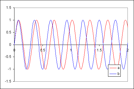
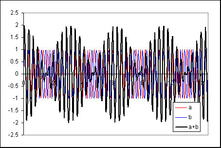
The force exerted (in the x-direction) by a rotating mass is sinusoidal. Because the two weights are rotated at slightly different speeds, the sinusoids have slightly different frequencies:


Side note:

The similar but non-identical speeds of these rotating weights can be easily designed by the use of gears. Shaft A (which holds mass a) can be connected to shaft B (which holds mass b) by a pair of gears. In the examples used here, the gear on shaft A has 22 teeth; the gear on shaft B has 20 teeth. A motor driving any of these shafts would drive both of them with the preset ratio of speeds.

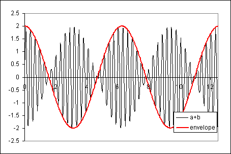
The combined effect of sinusoids of different frequencies (but identical amplitudes) exhibits a beating trend: the vibration frequency is the average of the two vibrations, while the beating frequency is the difference between the two vibrations.



Side note:

The centripetal/centrifugal force (F) associated with an eccentric weight of mass M, eccentricity e (distance from shaft centerline to centre of mass) and rotation speed ω is of the following form:
F = M × ω / e

Given that the force amplitudes of both shafts are to be the same,
F1 = F2, and hence
M1 × ω1 / e1 = M2 × ω2 / e2

The following figure shows the combined vibration with an envelope equivalent to the frequency difference between the rotating masses:


Later, when I was washing dishes, the complication of the vibrator problem revealed itself. The vibration amplitude not only pulsates in the x direction, but also in the y direction. What’s more, the pulsations in the x-direction are out of phase with the pulsations in the y-direction.

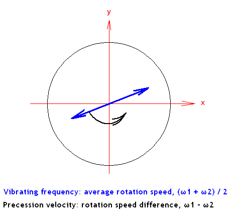
Restricting the analysis to the x-direction gives a severely misleading picture of the vibration behavior of this hypothetical Brrbrrbrr. When observed in 2 dimensions, the behavior of the vibration is rather interesting.

The direction of vibration precesses (rotates slowly), the rate of precession being equal to the speed difference of the two rotating masses.


This is what gives the pulsations in the x and y directions. As the direction of vibration rotates to coincide with the x-direction, the amplitude of vibration is the greatest in the x-direction. When the direction of vibration is perpendicular to the x-direction, there is no amplitude in the x-direction. Hence, the x-vibration pulsates.



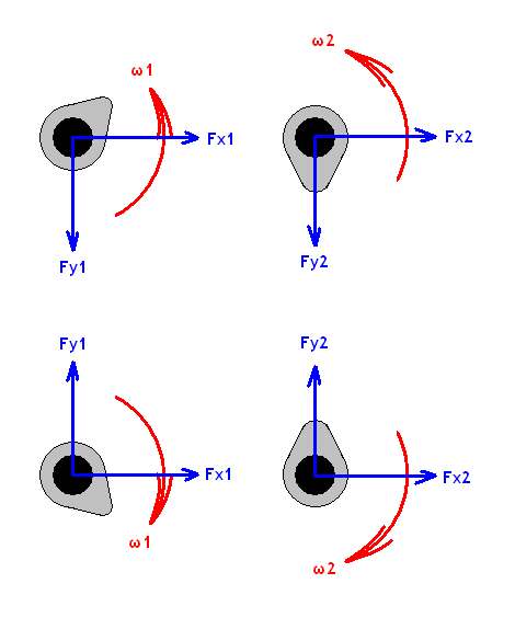
So it turns out that the pure pulsation I was searching for cannot be found in pairs of rotating masses. However, the pulsation can be restored by canceling vibrations in the y-direction, leaving only the x-direction to pulsate. This can be done by two pairs of rotating masses that rotate in opposite directions.


The arrangement shown above is designed so that the y-direction component of the centripetal forces are set up in opposing directions so that they contribute to a net of zero y-direction forces. But, the x-direction forces are arranged in the same direction, so that the x-direction vibration amplitude is doubled. And here, the analysis for uniaxial vibration (as presented above) can be applied, and pulsation is achieved.

Success!

Am I Yee Wei, who woke up from a dream in which I ate a goat, or am I a python dreaming I am surfing the web?
Which is real- the words, or the author?




I fly home on Saturday afternoon, and nothing has been packed.

The wedding is going to be interesting. The cousins have agreed to coordinate the colour of the clothes, hence expect a table full of pink and beige. Wickedness…

And my brother has secured the use of a huge Nikon SB-800 flashgun and a Canon EOS 650 camera body. Supplementing that to our existing collection of lenses, 3 camera bodies, a flashgun and suitable lens mount adapters, the extra body would help reduce time consuming lens changes.




On the basis of recommendations by 小李飞刀, I have laid my hands on a book by Lev Landau. It looks quite fantastic; the way in which he introduces special relativity is quite different from the typical SR text books.

The typical manner in which SR is introduced usually involves an experiment involving light bouncing around in a moving train. This tends to make (the speed of) light look like some kind of God-phenomenon that controlled the universe.

Landau did it the other way around, by introducing special relativity using an upper-limit on signal propagation velocities. And it turns out that electromagnetic radiation happens to ride on this very limit. The c that appears in the Lorentz-contraction is not explicitly the speed of light; it is the speed limit of signal propagation velocity.

An alternative interpretation of the measurement problem found in quantum mechanics

Assumed knowledge:
Some familiarity with Young’s double-slit experiment and quantum mechanical implications of the results.


One very fundamental problem in quantum mechanics is the ‘measurement problem’, in which the act of measurement itself is destroys interesting quantum effects.

The simplest example is using the two-slit experiment. The wave-like nature of light means that constructive and destructive interference result in the familiar fringes of light and dark bands.

If the light source’s intensity is reduced such that only photon is in the system at anyone time, as photon hits accumulate on the detector, the same fringes emerge. The obvious questions at this point are, "how is one photon interfering with itself? Did it go through both slits at the same time?"

Light detectors are then installed behind each of the slits, the objective being to identify which slit the photon actually went through. Unfortunately, and mysteriously, the interference pattern disappears.



Oftentimes, the explanation for this phenomenon is presented by invoking the Heisenberg Uncertainty Principle. On the other hand, Von Neumann and Weigner believed that it was the conscious observation that resulted in the collapse of a wavefunction. Still other interpretations claim that the experimental apparatus itself is part of the experiment, and the results show what the apparatus was designed to show: the wave-like or particle-like nature of light. The many-worlds interpretation raised by Everett is so radical that it is difficult for me to write his proposition succinctly.

However, I personally feel that these do not address the problem satisfactorily, and have developed a handwaving interpretation of my own, based on interactions and wavefunction collapse and reformation.



It would be appropriate to first describe the wavefunction in a general manner. In a handwaving way of explaining it, the wavefunction of a particle is a function that describes the probability of finding the particle in a particular location in space(time).

A wavefunction is said to collapse when the particle's position is 'revealed', so that it's position is no longer a probability distribution, but a definite point in space(time). At that moment, the probability of finding that particle is zero everywhere except where the particle is located.



We will now construct the experimental apparatus by considering the simplest case and incrementally adding elements of complexity to it to finally arrive at the double-slit set up with photodetectors.

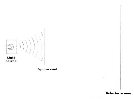
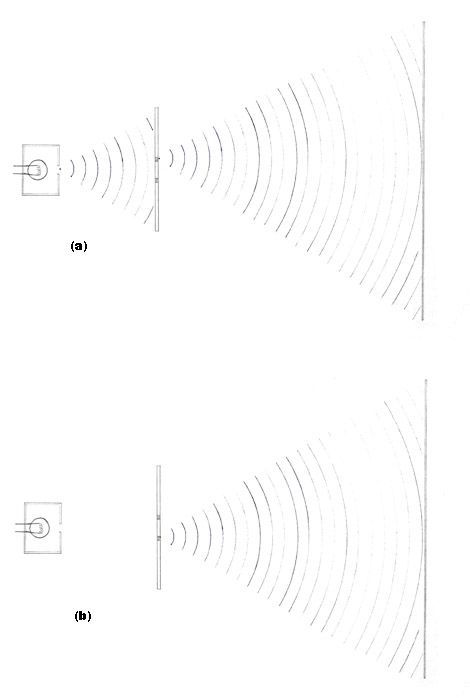
A light source, an opaque card (of sufficient thickness to prevent tunnelling effects) and a detector screen are arranged as in the double-slit experiment. However, the opaque card has no slits. All the light that is directed towards the card falls on the card’s surface.


Figure 1: No slits in the card; all light falls on the card’s surface.

From a wavefunction point of view, the wavefunction gives a probability of a photon striking a particular area of the card. When the photon strikes the (interacts with) card, it does so at one point, and the wavefunction has collapsed into a point at that location.

Also note that the presence of the opaque card has modified the wavefunction such that the probability of the photon striking the detector screen is zero.


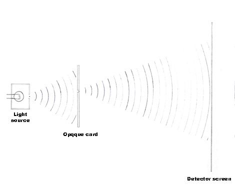
A slit is then cut in the card, and we see that while most light falls on the opaque card, some of it hits the detector screen.


Figure 2: One slit in the card; most light falls on the card's surface, but some reach the detector screen.

As one can see, the probability of finding the photon on the detector screen is no longer zero.


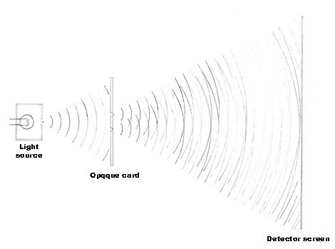
A second slit is cut into the card, and the detector screen shows the typical interference patterns that have become associated with the double-slit experiment.


Figure 3: Two slits in the card; most light falls on the opaque card's surface, but the light that falls on the detector screen has alternating light and dark bands that are characteristic to interference.



Photodetectors are then installed at the slits to observe which slit the photon 'actually' went through. The function of these detectors is to alert the experimenter when a photon passes through one of the slits. How the photodetector works is not of interest to us, but we can be sure that the photodetector has to interact with the photon if it is to send a signal that "yes, a photon has passed through."

And here comes the crux of my argument- interactions requires the whole photon’s participation (not merely the probability waves). Thus, only a wavefunction that had collapsed in the detector can produce an entire photon which is capable of interacting with the detector.


Name the photodetectors A and B. If A had sent a signal indicating the passage of a photon, this means that the photon had interacted with A (assuming that A is not faulty). The interaction means that the photon's wavefunction had collapsed into a point in the detector, manifested as the photon (a particle). The wavefucntion's collapse means that the probability of finding this photon on the opaque card or in photodetector B is zero- the photon is definitely in A, and thus definitely not in B nor on the opaque card's surface.

However our photodetectors are designed to allow the photon to proceed on its way to the screen, which means a new wavefunction is produced upon the old one’s collapse. The new wavefunction describes the propogation of a photon from detector A towards the screen. Since the wavefunction of a photon heading towards the screen comes from one source (detector A), there is no interference.


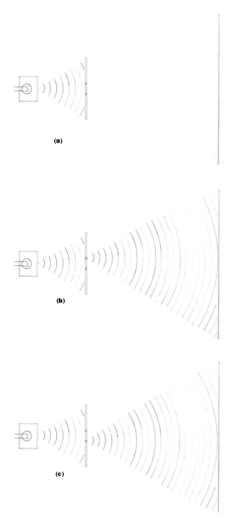
Figure 4:
(a) The photon strikes (interacts with) the opaque card, and the wave function collapses. This photon will never make it to the detector screen.
(b) The photon interacts with photodetector A, and the wavefunction collapses into the detector. The photon then continues on towards the screen, propagating as a new wavefunction originating from detector A.
(c) The photon interacts with photodetector B, and the wavefunction collapses into the detector. The photon then continues on towards the screen, propagating as a new wavefunction originating from detector B.


The interference pattern can also be made to disappear by using only one photodetector behind a slit. In this case, the initial wavefunction is such that there is a probability for the photon to strike the opaque card, strike the detector in the slit, or strike the screen. Any one of these interactions will cause the photon to exist as a particle, and the wavefuction to collapse.


Figure 5:
(a) The initial wavefunction shows that there is a probability for the photon to strike te opaque card's surface (which is not exciting), strike the detector screen (which is interesting) or interact with the photodetector hidden behind the lower slit (which is even more exciting).
(b) If the photon did interact with the photodetector in the lower slit, the initial wavefunction collapses, and a new wavefunction is formed. Note that there is no interference.


Thus the double-slit experiment and measurement problem has been explained by using the argument that an interaction requires the whole particle's presence, which means that the original wavefunction has to collapse, and a new wavefunction to propagate from that point.

It must be noted that the photodetectors behave similarly to the opaque card: it does not allow the wavefunction to have a non-zero value behind it. Hence, a photodetector absorbs photons, just like the opaque card. The difference lies in the fact that the photodetector then spits out that photon after having detected its presence. This new emission event corresponds to a new wavefunction.


Author's note:
Some feedback on the workability of this proposition please? Thank you.
Mr Lee, I'm counting on some sort of response from you.


Mathematics & Applied Sciences

A brief introduction to tidal forces

For me, the tides have been slightly troubling for as long as I can remember.

The most disturbing question was, why does high tide occurs on both sides of the earth in an elliptical shape, and not only the moon facing side?

The question was partially answered when I came across one of the last few chapters in 'Gravity: an introduction to Einstein’s general relativity'.


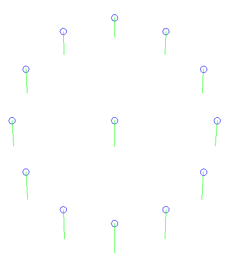
Consider a large array of small objects (mangoes, for example) freely falling towards a massive object (such as a star). Note that the separation of the individual mangoes is sufficiently large that the gravitational force and direction is not the same for all the mangoes.



At a particular time, the mangoes are arranged in a circular fashion with one of them in the middle as shown. The gravitational force vectors acting on the individual mangoes are also illustrated as arrows indicating the direction and magnitude.



As expected for gravitation, the relationship is proportional to the inverse of the square of distance. Thus, a greater force is exerted on mangoes nearer to the star than mangoes further away.

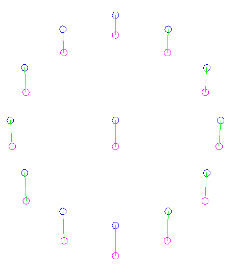
All the mangoes are accelerating towards the star. However, mangoes closer to the star experience a greater gravitational attraction towards the star, and thus accelerate faster towards the star. Similarly, mangoes further away accelerate slower. The end result is that the mangoes fall at different rates, and the circular array starts to deform. The circle stretches into an ellipse.



Apart from the forces’ magnitude, there is also a difference in force directions. The mangoes are all falling towards the centre of the star, but the mangoes are so far apart that they do not fall in parallel paths.

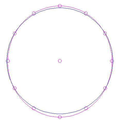
As a result of this converging nature of the free fall paths, the circle also narrows. The illustration shows the mangoes’ position at an interval after the time when they were arranged in the circular layout.

And thus the elliptical shape of the ocean’s tides has partly been explained. A more complete explanation will require that the moon and earth are orbiting each other as opposed to the radial plunge illustrated here using falling mangoes.


Blue curve: circle
Magenta curve: ellipse

Note that the force difference due to the moon is not particularly large; it causes a change in water level of only several metres, considering that the diameter of the earth is 12000 kilometres.

If an unfortunate person were to fall into a smallish black hole, the tidal forces near the singularity would be sufficient to tear the person apart. Parts nearer to the black hole accelerate dramatically faster than parts further away, the difference being sufficient to break the person into pieces.


Method for producing images:

AutoCAD was used to generate the images.
The circular array of mangoes has a radius of 4 units.
The distance between the centre of the array and the star is 60 units.
The distances between individual mangoes and the star were measured using the dimensioning tool
Gravitational attraction is proportional to the inverse of the square, thus this can be calculated from the measured distance.
For convenience, this gravitational force vector’s length was scaled arbitrarily such that the vector of force acting on the centre mango is 1 unit long.
Having determined the vector’s length on each mango, the vectors were drawn using the line tool.
The lines starts at the centre of each mango, and is pointed exactly at the centre of the star, and the line’s length adjusted accordingly.
The displaced positions of the mangoes are arbitrarily placed at the ends of the vector lines. This is acceptable for small time intervals (sufficiently small to neglect changes in gravitational force as the individual mango moves), since displacement s = 0.5at^t, and the displacements are all proportional to the vector lengths.
The final positions of the mangoes are exact, since they are derived as above.
The elliptical trend line is not an exact solution.


Mathematics, Physics

The length scales of the known universe

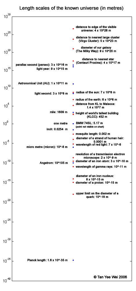
I find it difficult to appreciate the context of sizes involved when I read that the diameter of a proton is 0.000000000000001 metres, or that the diameter of our galaxy is 900000000000000000000 metres.

To ease this little problem, I took representative lengths from various orders of magnitude, sorted them in order, and arranged them on a logarithmic scale axis.

The numbers are written in what some refer to as ‘scientific notation’, where trailing (or leading) zeroes are condensed to a little exponent. For example,

0.0007 = 7 x 10^-4
3,750,000 = 3.75 x 10^6

The blue points correspond to length units other than metres, such as the mile, angstrom and light year. Their text markers are located left of the blue points.

The red points corresponds to lengths of objects, some familiar in our lives, mostly not.



Physics

A comparison between Newtonian and Relativistic models of simple oscillating systems

Special relativity will be discussed here, but it is best to learn special relativity from a proper text. While care has been taken to maintain accuracy, many of the important concepts in SR are not well represented here, especially the relativity part: relative to what?

A long time ago, I argued that rigid bodies do not exist. Here is a summary:

A rigid body’s length remains constant all the time. It cannot deform at all. Thus, when one pushes on one end of a rigid rod, the other end also moves at the same time. There is no delay between one end being pushed and the other end moving.

If we have a very long rod, and one end is pushed, at the same time, the other end will move. This process is instant.

However, a beam of light shined from the other end requires finite time to traverse the length of the rod. That being the case, it would seem that by pushing on long rods, information can be sent faster than the speed of light.

Of course, that is impossible. Thus, rigid bodies do not exist. Everything in this universe, from neutron stars to diamond gemstones, are not rigid; they are elastic. All of them.

Related links:
Rigid bodies violate special relativity
Real materials as opposed to rigid bodies

Rigid bodies are objects that have infinite stiffness. The question is, what sort of behaviour will be present when considering materials of large but finite stiffness?

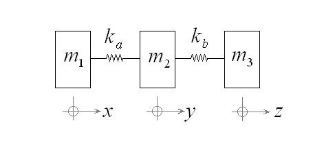
In taking a small step to answering this question, I have constructed a simple model of 3 masses m1, m2 and m3; connected by two linear springs of stiffness ka and kb. In this mathematical model, the coordinates for the individual masses, x, y, and z have their origins at the respective masses’ equilibrium positions.



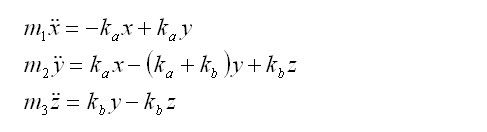
The differential equations of motion can be easily formulated using the simple F=ma relationship.

The differential equations for classical Newtonian mechanics are a set of 3 equations as such:



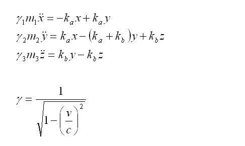
The system is then considered with Relativistic effects. The masses m1, m2 and m3 are called the rest mass, which is the mass measured when the system is stationary. As they move faster and faster approaching the speed of light, the measured mass becomes greater and greater, thus requiring more energy to accelerate. This is accounted for by a term γ that is multiplied with the rest mass.



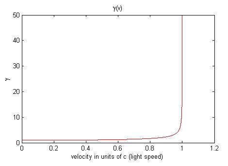
As one can observe from the above equation, when velocity v approaches the speed of light, γ approaches infinity. There is an infinitely high energy barrier that stands at the speed of light. Only massless particles, such as photons, may travel at light speed.

One important effect of γ on the equations of motion is that the mass becomes greater as speeds increase, such that the masses may never approach 300,000 km/s.


Having obtained the differential equations of motion, the motion is then simulated using the 4th order Rungge-Kutta algorithm with increment time intervals of 0.00001s.


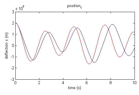
click here for a plot with a larger domain t=[0,20]
red: Newtonian
blue: Relativistic


The plots of the position of mass 1 using Newtonian and relativistic models are not significantly different to the naked eye.


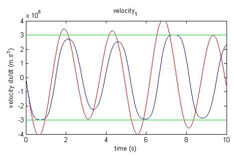
click here for a plot with a larger domain t=[0,20]
red: Newtonian
blue: Relativistic
green: light speed, c


However, the differences are clearly seen when the velocity plots are compared. The linear Newtonian model exhibits instances of violating the speed of light, while the relativistic one shows the energy barrier forbidding the speed to exceed 3x10^8 m/s.

Around the time of 1s, the Newtonian model shows speeds greater than c while the relativistic model remains bounded within c. Referring back to the position plot, this effect can be seen in the slope of the curves. The Newtonian model’s motion is faster, and the slope is thus steeper than the Relativistic model’s.

As a consequence, the frequency of oscillation in the relativistic model is lower than that present in the Newtonian model. Also, due to the nonlinear term γ, the Relativistic model does not exhibit sinusoidal motion.




Mathematics