Fun with the MoTeC data interpreter
What I did for Valentine’s Day:
Played GTR 2 for a few hours.
GTR 2 is a fearsomely realistic racing simulator based on the 2003 and 2004 FIA GT Championship series. While there are a huge number of bells and whistles, one of the most fascinating features of the game is the ability to save the car data into a MoTeC log file.
This is the same file format that a MoTeC data logger on an actual race car will produce: a time history of individual wheel speeds, suspension positions, suspension speeds, engine revs, throttle position, brake pedal pressure, steering angle, longitudinal acceleration, lateral acceleration, individual tyre temperatures at the inside, centre and outside areas…
And with the MoTeC data interpreter program, magic is possible.
***
The user can perform various mathematical operations on any combination the generous set of data logged by the MoTeC data logger.
For example, the instantaneous radius of curvature of the vehicle’s path can be calculated by rearranging the following equation:
a = v2/r
r = v2/a
Both the vehicle speed and lateral acceleration are measured, and so the radius can be determined.
Even more interesting, a general relationship between the vehicle’s speed and aerodynamic downforce can be observed after the data is suitably processed.
The principle objective of demanding greater aerodynamic downforce in a racing car is to allow greater acceleration (both in the longitudinal and lateral directions). Consequently, greater downforce will allow the vehicle to have higher accelerate.
From the logged longitudinal and lateral accelerations, the acceleration magnitude of the vehicle can be determined:
|a| = sqrt( along2 + alat2)
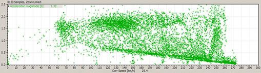
When |a| is plotted against vehicle velocity, the following scatter plot appears:
Click here for large size image
x axis: vehicle speed, v (km/h)
y axis: acceleration magnitude, |a| (g)
This plot consists of data recorded over a distance of 6 laps, equivalent to a duration of 13 minutes. Data was recorded at 10 Hz, producing 8130 data points.
Two general trends are visible:
the lower trend, consisting of a straight line that indicates a decreasing acceleration at higher speeds
the upper trend, indicating the maximum achievable acceleration increases when vehicle speed increases
The lower trend line corresponds to data recorded when the vehicle is accelerating on straight sections of the track. Given that the power output of the engine is maintained near the peak output (by adjusting the gearbox ratios to suit the track), the straight line is consistent with the fact that an object accelerated with a constant power will accelerate slower when the object is moving at a faster speed.
The upper trend is not as clear, but is nonetheless visible as an upward sloping trend.
At 60 km/h, |a| is approximately 1.75 g.
At 100 km/h, |a| is approximately 1.85 g.
At 160 km/h, |a| is approximately 2.10 g.
At 260 km/h, |a| is approximately 2.25 g.
Several data samples plot outside the upper trend because dips and bumps in the track will result in a different normal force acting on the wheels, thus allowing momentary increases and decreases in absolute acceleration.
A small cluster of data at 250 km/h show substantial deviation from the upper limit of acceleration. This, too, is caused by changes in track elevation where the main straight slopes upwards.
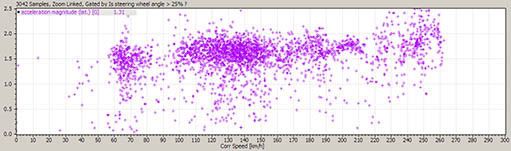
A similar plot can be produced showing lateral component of acceleration instead of total acceleration. In this case, |alat| was plotted against vehicle speed.
To prevent the chart from being cluttered with data not related to lateral acceleration (on straights, the lateral component of acceleration is close to zero), the plot was gated by plotting only data points that meet certain criteria.
Here, a new expression was defined, where
Steering = if (steering wheel angle > 25%) 1; else 0;
This expression will take the value 1 if there is substantial steering input, and 0 otherwise.
The criteria for gating the data is then set such that only data points with steering = 1 will be plotted, resulting in the scatter plot below:
Click here for large size image
x axis: vehicle speed, v (km/h)
y axis: lateral acceleration magnitude, |alat| (g)
This plot consists of data recorded over a distance of 6 laps, equivalent to a duration of 13 minutes. Data was recorded at 10 Hz, producing 8130 data points. Of these, 3042 data points satisfied the gating criteria and were plotted.
The |alat| plot resembles the |a| plot, except for the absence of the lower trend line. This is expected, because the lower trend line is associated with longitudinal acceleration driven by the vehicle’s engine.
A trend line indicating the upper bound of acceleration magnitude was constructed by approximation, and the following correlation appears:
|a|max = 0.0017 V + 1.56,
The units for |a|max and V are g and km/h respectively.
With the correlation between maximum |a| and vehicle speed approximated, a new variable called theoretical max acceleration was defined
theoretical max acceleration = 0.0017 vehicle speed + 1.56
This variable indicates the maximum acceleration that the vehicle tyres can provide.
When the instantaneous values of the theoretical max acceleration is compared against the actual accelerations, it can show areas where the driver can improve his/her lap time. For example, it can reveal that the driver can apply the brakes slightly later and harder on entry into a particular corner, thus shaving several milliseconds from the lap time; or that the vehicle can move slightly faster at a particular curve without exceeding the traction limits of the tyres.
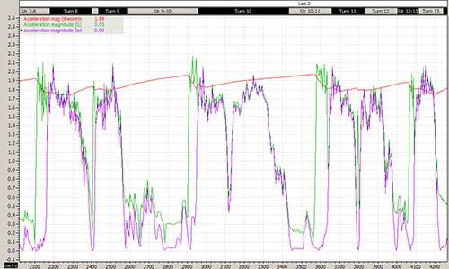
In the following graph, theoretical max acceleration is plotted together with actual |a| and |alat| in the upper graph. The max theoretical acceleration approximates the shape of the peak accelerations but is not accurate due to the coarse approximation for the speed and downforce correlation.
Click here for large size image
x axis: distance (m)
y axis: theoretical max acceleration, |a| and |alat| (g)
This plot consists of data recorded over a distance of 2.8 km. Data was recorded at 10 Hz, producing 631 data points.
Played GTR 2 for a few hours.
GTR 2 is a fearsomely realistic racing simulator based on the 2003 and 2004 FIA GT Championship series. While there are a huge number of bells and whistles, one of the most fascinating features of the game is the ability to save the car data into a MoTeC log file.
This is the same file format that a MoTeC data logger on an actual race car will produce: a time history of individual wheel speeds, suspension positions, suspension speeds, engine revs, throttle position, brake pedal pressure, steering angle, longitudinal acceleration, lateral acceleration, individual tyre temperatures at the inside, centre and outside areas…
And with the MoTeC data interpreter program, magic is possible.
The user can perform various mathematical operations on any combination the generous set of data logged by the MoTeC data logger.
For example, the instantaneous radius of curvature of the vehicle’s path can be calculated by rearranging the following equation:
a = v2/r
r = v2/a
Both the vehicle speed and lateral acceleration are measured, and so the radius can be determined.
Even more interesting, a general relationship between the vehicle’s speed and aerodynamic downforce can be observed after the data is suitably processed.
The principle objective of demanding greater aerodynamic downforce in a racing car is to allow greater acceleration (both in the longitudinal and lateral directions). Consequently, greater downforce will allow the vehicle to have higher accelerate.
From the logged longitudinal and lateral accelerations, the acceleration magnitude of the vehicle can be determined:
|a| = sqrt( along2 + alat2)
When |a| is plotted against vehicle velocity, the following scatter plot appears:
Click here for large size image
x axis: vehicle speed, v (km/h)
y axis: acceleration magnitude, |a| (g)
This plot consists of data recorded over a distance of 6 laps, equivalent to a duration of 13 minutes. Data was recorded at 10 Hz, producing 8130 data points.
Two general trends are visible:
the lower trend, consisting of a straight line that indicates a decreasing acceleration at higher speeds
the upper trend, indicating the maximum achievable acceleration increases when vehicle speed increases
The lower trend line corresponds to data recorded when the vehicle is accelerating on straight sections of the track. Given that the power output of the engine is maintained near the peak output (by adjusting the gearbox ratios to suit the track), the straight line is consistent with the fact that an object accelerated with a constant power will accelerate slower when the object is moving at a faster speed.
The upper trend is not as clear, but is nonetheless visible as an upward sloping trend.
At 60 km/h, |a| is approximately 1.75 g.
At 100 km/h, |a| is approximately 1.85 g.
At 160 km/h, |a| is approximately 2.10 g.
At 260 km/h, |a| is approximately 2.25 g.
Several data samples plot outside the upper trend because dips and bumps in the track will result in a different normal force acting on the wheels, thus allowing momentary increases and decreases in absolute acceleration.
A small cluster of data at 250 km/h show substantial deviation from the upper limit of acceleration. This, too, is caused by changes in track elevation where the main straight slopes upwards.
A similar plot can be produced showing lateral component of acceleration instead of total acceleration. In this case, |alat| was plotted against vehicle speed.
To prevent the chart from being cluttered with data not related to lateral acceleration (on straights, the lateral component of acceleration is close to zero), the plot was gated by plotting only data points that meet certain criteria.
Here, a new expression was defined, where
Steering = if (steering wheel angle > 25%) 1; else 0;
This expression will take the value 1 if there is substantial steering input, and 0 otherwise.
The criteria for gating the data is then set such that only data points with steering = 1 will be plotted, resulting in the scatter plot below:
Click here for large size image
x axis: vehicle speed, v (km/h)
y axis: lateral acceleration magnitude, |alat| (g)
This plot consists of data recorded over a distance of 6 laps, equivalent to a duration of 13 minutes. Data was recorded at 10 Hz, producing 8130 data points. Of these, 3042 data points satisfied the gating criteria and were plotted.
The |alat| plot resembles the |a| plot, except for the absence of the lower trend line. This is expected, because the lower trend line is associated with longitudinal acceleration driven by the vehicle’s engine.
A trend line indicating the upper bound of acceleration magnitude was constructed by approximation, and the following correlation appears:
|a|max = 0.0017 V + 1.56,
The units for |a|max and V are g and km/h respectively.
With the correlation between maximum |a| and vehicle speed approximated, a new variable called theoretical max acceleration was defined
theoretical max acceleration = 0.0017 vehicle speed + 1.56
This variable indicates the maximum acceleration that the vehicle tyres can provide.
When the instantaneous values of the theoretical max acceleration is compared against the actual accelerations, it can show areas where the driver can improve his/her lap time. For example, it can reveal that the driver can apply the brakes slightly later and harder on entry into a particular corner, thus shaving several milliseconds from the lap time; or that the vehicle can move slightly faster at a particular curve without exceeding the traction limits of the tyres.
In the following graph, theoretical max acceleration is plotted together with actual |a| and |alat| in the upper graph. The max theoretical acceleration approximates the shape of the peak accelerations but is not accurate due to the coarse approximation for the speed and downforce correlation.
Click here for large size image
x axis: distance (m)
y axis: theoretical max acceleration, |a| and |alat| (g)
This plot consists of data recorded over a distance of 2.8 km. Data was recorded at 10 Hz, producing 631 data points.
Labels: applied mathematics, applied science, how-to, physics
posted by Tan Yee Wei at 2/15/2009 12:40:00 pm
![]()
![]()

<< Home