e - unifying two common definitions of e

Note: The concept of infinity would be used liberally here. For a brief introduction to the origins of the infinities found in today's context, read this post.


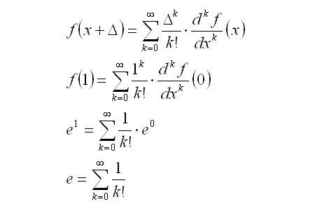
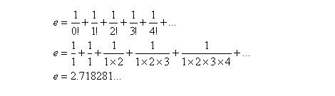
Perhaps the most common expression that gives the value of e would be the sum of the reciprocal of factorials, from zero to infinity.

Equation (1)

Another well known expression is:

Equation (2)

I will attempt to show that these two expressions are identical. Firstly, I will let a be a finite number before pushing it towards the great infinity.

Equations (3)

Here, a takes the value of 4. Expanding the brackets, we see that the terms are results of multiplication between 1 and ¼. In the last line above, the coefficients 1, 4, 6, 4, 1 are actually binomial coefficients resulting from 4C0, 4C1, 4C2… 4C4.

For example, 4C2=6 arises because (¼)^2 appears 6 times as a result of the 6 different ways the terms can combine to give (¼)^2. The combinations are:

Multiply ¼ from the 1st and 2nd brackets, and multiply with 1 from the 3rd and 4th brackets.
Multiply ¼ from the 1st and 3rd brackets, and multiply with 1 from the 2nd and 4th brackets.
Multiply ¼ from the 1st and 4th brackets, and multiply with 1 from the 2nd and 3rd brackets.
Multiply ¼ from the 2nd and 3rd brackets, and multiply with 1 from the 1st and 4th brackets.
Multiply ¼ from the 2nd and 4th brackets, and multiply with 1 from the 1st and 3rd brackets.
Multiply ¼ from the 3rd and 4th brackets, and multiply with 1 from the 1st and 2nd brackets.

If you have no idea what I am talking about, try expanding f(6) into individual terms. It should become clear after that.

f(a) can then be rewritten as

Equations (4)

Expressing the binomial number as a ratio of factorials gives the final line in Equations (4).

Substituting f(a) into the definition of e (equation 2):

Equations (5)

The equation is beginning to resemble the infinite sum of inverse factorials:

Equations (6)

To show that these equations are equivalent, the following expression needs to be true:

Equations (7)

When a approaches infinity, the terms in the brackets should converge to unity, and the expressions in equations (6) would be identical.

Expanding the terms in the bracket:

Equations (8)

Cancelling terms that appear in the numerator and denominator:

Equations (9)

Note that there are an equal number of terms in the numerator and denominator. For (a-n)!, the missing terms are replaced with the a^n.

Replacing this result into the previous expression:

Equations (10)

When taking the limit of a approaching infinity, (a-k)/a is unity regardless of the value of k. After all, infinity minus 5 is still infinity.

Thus, it summary

Equations (11)

One very valid concern is, “what happens when k ≈ a? When k ≈ a, (a-k)/a is no longer unity and equation (6) might not match term-for-term.”

Fortunately, this never happens. Observe how the equation is structured: first, let a approach infinity. Then, incrementally increase n and k.

n and k can be as humongous as one wishes to make it, but they would always be dominated by a. You can even make n and k as large as the second Skewe’s number, and they would still not make a dent in a. The second Skewe’s number is finite; a is not.

Real numbers – the slippery slope to insanity

Let’s build real numbers from scratch using the Dedekind cut. Use the square root of 2 as an example. Does √2 exist? Specifically, is there an x that can satisfy the equation x^2 = 2 (x squared = 2)?

As the Ancient Greeks already knew, x is definitely not a rational number (fractions and whole numbers). With an understanding that extends only to the rational numbers, how can x be created using and building from existing knowledge?

To perform the Dedekind cut, group all the rational numbers into two sets a and b as follows:
a = {x : x^2}
b = {x : x^2 > 2}

The set a contains all the rational numbers that are less than two when squared; b is the opposite. A few of the elements in a and b are:
a = {1.03, 0.2432, -1.2, …}
b = {3.5, 2.72, -342.22, …}

I must stress this again: all elements in a and b are rational numbers. We currently trying to construct the concept of real numbers from rational numbers.

Interestingly, there is no largest element in a. Give my any element in a and I can find you another element (still in a) that is larger than yours, despite the constraint imposed upon by the rule that all elements in a must obey x^2 a is constructed (it only has elements that squares to less than two), all elements in a will never exceed a certain value. For example, the elements in a will definitely not exceed 19, because 19 squared is 361, definitely greater than 2. We say that 19 is an upper bound of a. No element in a exceeds 19.

But 19 is a very boring upper bound for a. It is like saying "the population of China is definitely less than 27 trillion." Duh.

We can use a smaller value for the upper bound of a, maybe 12. 12 squared is 144, which is greater than 2. For sure, no element in a will be greater than 12.

The upper bound of a can be made smaller and smaller, using 10, 7.4, 5.4, 3.5, 1.5…

And here comes the crucial step: the least upper bound of a is the square root of 2. From two groups of rational numbers, we have conjured a real number.

Recall that there is no largest element of a. Similarly, there is no smallest element of b (ignoring the signs). Like in the previous illustration, we can write a list of elements of b, all of them decreasing and there would never be a smallest element.
5.4
2.54
2.1
1.5
1.46
1.4149
1.4142135626

Interestingly, the least upper bound of a does not lie in a and does not lie in b (after all, a and b can only contain rational numbers). The definitions of sets a and b leave an infinitesimally small gap between them, a gap that can only fit one (real) number- √2.

And that’s all there is to creating real numbers from rationals. It probably feels a little inadequate, a little unsatisfying- as if the real number was not properly created. But bear in mind that the Dedekind cut is merely creating the concept of real numbers. It tells us that the square root of two is not some dodgy product of black magic, but is in fact a very real number.

What the Dedekind cut does not do is tell us the value of √2. It cannot do that. Nothing can- our only understanding of √2 is that it satisfies the equation x^2=2.

We can make approximations (x ≈ 1.4142135624 ), we can generate algorithms to tell us the 96 millionth digit in √2, but we can never know the exact value of √2- it has infinitely many digits.



Mathematics & Applied Sciences

A brief explanation of the Taylor Series via the Mean Value Theorem

Assumed knowledge: some tertiary level calculus

Introduction

This article will explain the Taylor series by using the mean value theorem. The mean value theorem will be explained in a general manner before the proceeding on to the Taylor series.

The Taylor series will not be rigorously derived.


The mean-value theorem

For any continuous and differentiable function in the interval (x1,x2), there exists at least one point between x1 and x2 such that


equation (1)

In other words, there is at least a point on the function between the two points that has slope equal to the slope between the two points x1 and x2.

2 graphs illustrate the point. Note the parallel lines.



While the mean value theorem may appear intimidating at first, it is conceptually identical to the idea presented below.

For a continuous function f, there exist a point ξ between x1 and x2 such that f(ξ) is the average of f(x1) and f(x2)


equation (2)



f(x1) and f(x2) are on different sides of the average f(ξ), and since the connection between f(x1) and f(x2) is continuous, this imples that there MUST be a point where the line crosses the average value.


The Taylor Series

The Taylor series is an expansion of a function about a point.


equation (3)

Using the mean value theorem, we can say that there exists a point ξ(1) between x and x+Δ that has slope equal to the slope of the line between the function values of x and x+Δ.

The expression of f(x+Δ) can then be written as follows:


equation (4)

Again, note that the slope at ξ(1) is equal to the slope between the function values of x and x+Δ.


Now, for the most exciting part of this expansion. We will apply the mean value theorem onto the derivative in equation (4).


equation (5)

Repeating the above step for the second derivative:


equation (6)

This step can be applied indefinitely onto higher and higher derivatives, and the result would be as follows:


equation (7)

For equation 7 to be equal to equation 3, the following would be true:


equation (8)

Unfortunately, equation 8 is not as easy to derive/proof as its simplicity may otherwise suggest. As such, this article would end here.


Mathematics

Finding the value of e

Euler’s number, e, is special in many ways. The exponential function of e is particularly fascinating in that the slope of the function at any point is equal to the function value at the point.




Since this is an exponential function, it should be reasonably easy to see that
f (0) = 1
f (1) = e

But what is the value of e?


Assuming the truth of the Taylor Series expansion of a function:



If we were to substitute the exponential function into the Taylor series, and let x = 0 and Δ = 1, then:



And there it is! The value of e is the sum of all the inverses of factorials. Expanding the summation:






Mathematics